Staying within the boundaries of grade-school mathematics, we now turn to averages. Recall that you were taught that there are three kinds of averages:

1)  the mean or, more technically, the arithmetic mean (the sum of the values divided by the number of cases—what we usually intend when we use the term "average" in everyday conversation);

2)  the median (the midpoint in a range of values so that half of the values are higher and half are lower); and

3)  the mode (the most often repeated value within a data set).

All three kinds of averages are measures of what statisticians call "central tendency." That is, they represent an effort to identify the center or central number within a range of data, thereby summarizing what the data have in common.

Let’s look at an example of historical analysis that uses averages. Our data set is drawn from the tax list of Russia Township, Ohio, in 1850. The tax list provides property assessments for a total of 392 resident taxpayers. With the help of Microsoft Excel, we have calculated the mean, median, and mode:

Mean=$667
Median=$389
Mode=$260

What was the "typical" property assessment in Russia Township, Ohio, in 1850?

$260
$389
$667

Why the median and not the mean or the mode? Each of these figures tells us something about the average property holding of a Russia Township taxpayer in 1850. Indeed, depending on what you intend by the term "typical," you could argue that the typical Russia Township taxpayer owned $260, $389, or $667 in assessed property in 1850. 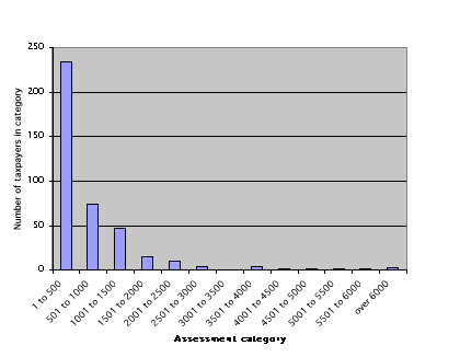It is important to specify which measure you are using when you speak of the "average" or "typical" member of a data set.

Taken together the mean and median tell us something about the larger pattern of property holding in Russia Township that neither reveals on its own. From the fact that the mean is higher than the median, we can infer that the distribution of property assessments is skewed rather than symmetrical. As it happens, the assessments of a small number of quite large property holders raised the mean without affecting the median. This pattern is visually evident in the following graph of the distribution of property assessments:

Graph 3: Distribution of Taxpayers by Assessment Category, Russia Township, Ohio, 1850

As Graph 3 makes clear, there was a large range of property assessments in Russia Township in 1850. And just as averages summarize the central tendency of a data set, other measures are useful for summarizing the dispersion or variability of a data set. The simplest way to specify dispersion is to give the minimum and maximum of the range, $13 and $7358 in the case of Russia Township property assessments. But the minimum and maximum by themselves do not tell us much about how tightly clustered or broadly spread out the bulk of data points are; they just tell us where the extremes lie at either end of the range.

A less intuitive but otherwise more useful summary statistic of dispersion is standard deviation. Technically, standard deviation is defined as "the square root of the arithmetic mean of the squared deviations from the mean"*, and it is calculated according to the following formula:

If this seems a bit confusing, don’t panic. For common sense purposes, you may wish to conceptualize standard deviation in one of three ways. The first is to think of it as a measure of the average of the distances between each data point and the mean of the data set. The standard deviation is not the mean of the distances of the data points from the mean, but it is a kind of average.

A second way to think about standard deviations requires that you imagine a normal distribution or the so-called bell curve as pictured below. You are probably familiar with the notion of a normal distribution because aptitude and achievement tests like the SAT are designed so that test scores will be distributed according to such a symmetrical pattern within a large population.

Statisticians have established that in all normal distributions approximately 68 percent of the data will fall within one standard deviation on either side of the mean, and approximately 95 percent of the data will fall within two standard deviations on either side of the mean. That does not mean all normal distributions are identical, however. The bell curve can be flatter or steeper depending on the relative dispersion of the data. If the data are spread out, then the curve will be flatter and the standard deviation larger. If the data are tightly clustered around the mean, then the curve will be sharper and the standard deviation smaller. But the proportion of data within one standard deviation (68 percent) and within two standard deviations (95 percent) remains the same across all normal distributions. (Click to see an example of what happens to a normal distribution curve when you change the standard deviation. This link will take you to Berrie's Statistics Page and requires Quicktime player.)

Unfortunately, historical data rarely arrange themselves neatly into a normal distribution. So you may want to think about standard deviation in a third way, by comparing its magnitude to the mean of the data set. As a rule of thumb, when the standard deviation is smaller than the mean, the data are relatively closely clustered and mean is considered a reasonably good representation of the full data set. By contrast, if the standard deviation is greater than the mean, then the data are relatively widely dispersed and the mean is a rather poor representation of the full data set.

If we return to the data set of Russia Township taxpayers in 1850, we can calculate the standard deviation with the help of Microsoft Excel. It is $907, considerably larger than the mean of $667. Here is further evidence that it would be misleading to say, "The typical Russia Township taxpayer was assessed for $667" just because the mean property assessment was $667. In this instance, a better measure of typicality would be the median: $389.